Why I did this
I read Ryan Orbuch’s essay Natural General Intelligence about how much data we collect about the Earth. Most of it comes from physical sensors measuring nature and I got curious about how that data becomes something we can learn from. That led me to WeatherBench 2 and a lot of science and terms I didn’t know so I decided to learn it by building something.
The goal
I gave myself one dataset to own from end to end. Four years of hourly readings from about 165 California weather stations would go from NOAA’s raw public archives to a training-ready table with a quality verdict (pass, suspect or quarantine) on every value. Then I’d find out how often those verdicts are right and whether they actually make a model better.
When that worked I added radar as a second and very different sensor and pushed a 27 GB grid of the HRRR weather model through the same pipeline to see what changes with scale. Everything ran on a 16 GB laptop.
Getting to know the data
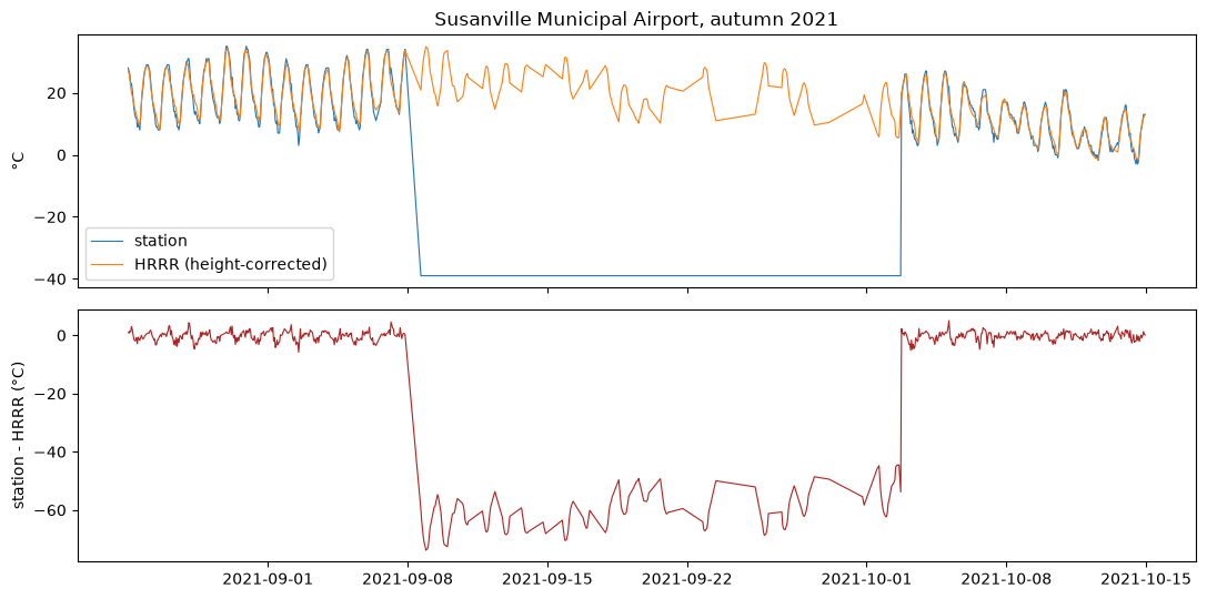
I started with the smallest stream on that chart. NOAA keeps every airport weather report as text and an hour can hold several of them taken at different minutes so even “the temperature at 2 pm” needs a written rule. NOAA’s own quality flags were the bigger surprise. They passed a sensor stuck at −39 °C for most of a month and marked four years of a healthy station as erroneous.
That raised the obvious question of what to compare a thermometer against. I used the HRRR weather model’s one-hour forecast and not its analysis because the analysis has already been nudged toward these same stations. Where the two disagreed there was usually geography behind it. Coastal stations ran warm because the model’s grid box holds sea and high valleys ran cold because cold air pools there at night.
Radar was the second sensor and about 300 times bigger. Its beam climbs as it goes out because the Earth curves away underneath it. It also hears more than rain.
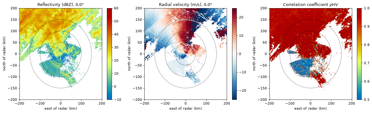
Matching four years of radar rain against station gauges showed how much the beam height matters. Radar saw about 90% of the gauge rain where its beam passed low over a station and less than half where it passed more than 2 km up.
Teaching myself to catch bad data
A quality check is a classifier and I wanted to measure it like one. Real data has no labels though. For recall I broke clean stations on purpose and kept an answer key (steps, drifts, biases, stuck values, clocks hours off and gaps only during storms). For precision I checked 30 real alarms by hand.
Loud faults were easy. A 2 °C step was found almost every time and a 0.5 °C step almost never. Most real false alarms were weather (coastal heat waves, Santa Ana winds the model timed an hour off and valley fog) and the checks found four broken sensors NOAA had passed.
Does it help a model?
I trained a gradient-boosted model that corrects HRRR at each station on several versions of the same training data and tested every version on a clean 2024.
| Training data | Error at the broken stations (°C) |
|---|---|
| Clean | 1.14 |
| No model, just HRRR | 1.45 |
| Broken | 1.57 |
| Broken with flagged hours removed | 1.52 |
| Broken with the same number of hours removed at random | 1.57 |
| Broken with shifted stretches repaired | 1.17 |
Broken data made the model worse than having no model because it learned each broken station’s offset faithfully. Removing the flagged hours barely helped since most of the damage came from stations reading a degree or two off for months. What worked was finding the dates where a station’s level shifted and correcting the stretch before it.
Designing it for petabytes
My data is a few GB. I wanted to think through how the same pipeline would work if it had to take in every radar, station and model run in the country with years of history behind them. I haven’t run anything at that scale so this is how I’d expect to build it and where I’m unsure. It follows one radar file from the moment it lands to the moment a model reads it.
Getting data in
Each of the roughly 160 US radars writes a new file every 4 to 10 minutes into NOAA’s public bucket on AWS. The bucket announces every new file as a notification so nothing has to poll for it. I’d point those notifications at a queue that sits between files arriving and files being processed. When a storm triples the rate of files the queue just gets longer for a while instead of overwhelming the workers. A message that fails can be retried.
A planner reads from the queue and groups files into units of work. For radar a unit might be one radar for one hour. Before running a unit the planner asks the manifest whether it has already been done. The manifest is a small database table with one row per unit. It records which input files the unit used, which version of the code ran it, whether it finished and where its output went. If the same unit already finished with the same inputs and code it’s skipped and that makes a file announced twice harmless. When the code changes the manifest also says exactly which units have to run again.
Workers pick up the units, read the files straight from the bucket and write their output. They’d run in the same region as the bucket so reading is fast and cheap. History goes in the same way. A backfill job lists the old files and sends the same kind of messages so four years of history runs through exactly the same code as a file that landed a minute ago. I think it needs its own lower-priority queue though. Otherwise a four-year backfill would sit in front of live data for days.
Laying it out
What a worker writes depends on the shape of the data. A station file becomes rows in a table. Each row is one station-hour with the value in SI units and UTC along with NOAA’s quality code and the time the report was really taken. The table is stored as Parquet in a folder per year with one file per station inside it. A year of about 3,000 US stations is then one folder of about 3,000 files with thousands of rows each. That keeps common questions to a few files and avoids millions of tiny ones.
Model grids go into Zarr. Zarr is a format for large arrays that cuts an array into chunks and stores each chunk as its own compressed object, with a small JSON file describing the whole array. For HRRR I’d try chunks of one day by a 512 × 512 tile (about 25 MB each). That should be big enough for object storage to handle efficiently and small enough to fetch on its own. The raw files are never edited so every one of these layers can be rebuilt from them if a rule or a bug changes.
When data arrives late
From what I read not everything arrives on time. Some ocean buoys are only read when a ship visits and NOAA notes that values and their quality flags in its station archive can change as late data comes in (GHCN-Daily). I’m not sure how often that happens for the stations I used. If it does it matters most for checks that compare a station with its neighbours. A QA run on 3 January might judge an hour when only three of five neighbours have reported and call it a pass. Once the other two arrive the comparison changes and the run on 5 January marks the same hour suspect. When I replayed my own checks month by month (notebook 06) 1.7% of verdicts changed like this. So I wouldn’t overwrite QA results. Each run writes its results beside the last one and each training run records which QA run it used. A model can then always be traced back to the exact verdicts it trained on.
Reading it back
Different readers ask different questions. A training job reads whole maps one hour at a time while an analyst might want four years at a single place. With chunks shaped like maps the training job’s hour is one chunk but the analyst’s four years is over a thousand. With chunks shaped like long time series it’s the other way round. I measured this on four years of HRRR over California stored both ways and the difference was 200 to 450 times for the same data on the same disk. So I’d keep a copy for each kind of reader. Either way nothing gets loaded whole. A cluster in the same region as the bucket reads only the chunks a question needs and reduces them to something small like a mean before sending it back.
There’s a lot here I’m still learning. I don’t know yet when a day of data should count as final, how to tell a quiet format change at the source from a real change in the weather or how fast chunked data can be shuffled to keep a training job busy.
What I took away
Every number in this project had a reason behind it that lived in the domain: why a station runs warm, why radar misses the rain under its beam, why a verdict changes a month later. I keep running into how much there is to know before the data makes sense and each answer opened two more questions. That’s the part I want to keep going deeper on, both the science of these natural systems and how to engineer for them.
The notebooks
| # | Notebook | The question it answers |
|---|---|---|
| 01 | Stations: read and explore | what does a station actually report? |
| 02 | Radar: read and explore | how does a radar see and what fools it? |
| 03 | Matching to a reference | what can a thermometer be compared against? |
| 04 | How data goes wrong | what do real sensor faults look like? |
| 05 | QA checks and metrics | how often are the verdicts right? |
| 06 | Monitoring and verdicts | do verdicts change over time? |
| 07 | Pipelines with Ray | how do I rerun everything safely? |
| 08 | Spark and Beam | what is each framework built for? |
| 09 | Does clean data help the model? | does any of this matter to a model? |
| 10 | Radar vs gauges | when do two rain sensors disagree and why? |
| 11 | Gridded data at scale | what does chunk shape cost? |
Sources: NOAA ISD, HRRR, NEXRAD and MRMS on AWS · Orbuch, Natural General Intelligence · Rasp et al., WeatherBench 2 · NWS ASOS · HRRR run lengths · rechunker.